
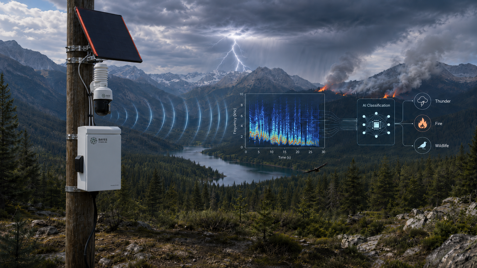
Integrated Acoustic Monitoring & Prediction System:Lightweight Edge-Deployable Environmental Sound Classification
Abstract
This paper presents an integrated acoustic monitoring system designed for real-time environmental sound classification on edge devices, with a focus on thunder and fire detection in mountain ecosystems. The system addresses the challenge of deploying reliable, always-on acoustic monitoring under strict computational and power constraints, without dependence on cloud infrastructure. A corpus of 4,041 audio clips spanning six environmental sound classes was assembled from two public datasets and one custom-assembled dataset: ESC-50, FSD50K, and a custom FireDataset. Four feature extraction strategies were systematically evaluated, culminating in a novel audio tiling approach that eliminates zero-padding artifacts by looping audio segments to fill fixed-length chunks. Three lightweight model architectures were trained and compared: a 2D convolutional network inspired by BC-ResNet, a 1D temporal convolutional network based on MatchboxNet, and a recurrent model using Gated Recurrent Units (GRU). The best-performing configuration, BC-ResNet with 5-second tiled mel spectrogram chunks, achieved 82.6% overall test accuracy and 88% Thunder recall with approximately 50,000 parameters and an estimated 50ms inference latency on a Raspberry Pi 4. The results demonstrate that lightweight convolutional neural networks, combined with thoughtful audio preprocessing and class balancing strategies, can serve as practical always-on acoustic monitors for natural environments.
1. Introduction
Acoustic monitoring of natural environments has emerged as a critical tool for ecological research, disaster prevention, and wildlife conservation. Mountain ecosystems in particular are subject to rapidly changing environmental conditions, including lightning strikes, wildfires, and extreme weather events that pose significant risks to both human safety and biodiversity. Traditional monitoring approaches rely on dedicated sensor networks with centralized data processing, introducing latency, infrastructure cost, and single points of failure. Edge-deployable machine learning systems offer a compelling alternative: lightweight models capable of running continuously on constrained hardware with no network dependency.
This project develops and evaluates an Integrated Acoustic Monitoring and Prediction System (IAMPS) targeting two primary detection tasks: lightning and thunder detection from acoustic signatures, and the foundational classification infrastructure for biodiversity monitoring through animal vocalization identification. The system is designed to operate as a Keyword Spotting (KWS)-style always-on detector, analogous in architecture and constraint to commercial wake-word detection systems, rather than as a conventional offline Environmental Sound Classification (ESC) pipeline.
The central research questions addressed in this work are:
Which feature extraction strategy best captures the acoustic characteristics of environmental sound classes under edge deployment constraints?
Which lightweight model architecture achieves the best balance between overall accuracy, class-specific recall (particularly for Thunder), and computational efficiency?
Can audio tiling as a preprocessing strategy improve model performance relative to zero-padding for variable-length audio classification?

2. Background and Related Work
2.1 From ESC to Streaming Edge AI: A Reframing
Initial literature review for this project focused on Environmental Sound Classification (ESC) research, which provided essential foundations in feature representation, CNN architectures, and evaluation methodology. However, a critical realization emerged during the review process: ESC research implicitly assumes conditions that do not hold in a real-world always-on system. ESC papers typically assume fixed-length audio clips, offline or batch inference, one classification decision per clip, and accuracy as the primary metric. These assumptions break down in the target application, where audio is continuous and unbounded, target events are rare, the system must run 24/7, false positives accumulate over time, and hardware and power are strictly constrained.
This realization motivated a reframing of the project around Keyword Spotting (KWS) literature, which addresses system-level concerns that ESC research abstracts away. Structurally, thunder detection is analogous to wake-word detection, a rare, acoustically distinctive event that must be reliably identified in a continuous stream with minimal false triggers. This reframing informed all subsequent architectural and preprocessing decisions.
2.2 Environmental Sound Classification Foundations
Piczak (2015) introduced the ESC-50 dataset [20] and demonstrated that 2D CNNs operating on log-mel spectrograms outperform traditional hand-crafted feature classifiers for environmental sound classification, establishing the spectrogram-CNN paradigm that dominates subsequent work [1]. Salamon and Bello (2017) extended this finding, showing that deep CNNs combined with audio data augmentation achieve state-of-the-art performance on UrbanSound8K even when labeled data is limited [2]. Their work directly motivates the use of mel spectrogram features as the primary representation in this project.
Mushtaq and Su (2020) conducted a systematic comparison of CNN architectures and feature representations on ESC-10, ESC-50, and UrbanSound8K, finding that CNNs without max-pooling using log-mel features with offline data augmentation achieve the best results, 94.94% on ESC-10 and 89.28% on ESC-50 [3]. Their work confirms that feature design and regularization choices are often more impactful than architectural complexity.
Li et al. (2017) compared deep learning and traditional approaches for environmental sound detection on the DCASE 2016 dataset, finding that late fusion of complementary models yields the best performance (~88% accuracy) and that no single model dominates across all feature types [4]. This finding informed the decision to evaluate multiple architectures rather than committing to a single model family.
Zhang et al. (2017) proposed dilated convolutional neural networks for ESC, demonstrating that dilated convolutions capture long-range temporal context more efficiently than deeper standard CNNs while maintaining comparable computational complexity [5]. Their work achieves 81.9% on UrbanSound8K and motivates the consideration of receptive field design in our architecture selection.
2.3 Bioacoustic Monitoring
For the biodiversity monitoring component of the project, several bioacoustic-specific works were reviewed. Kahl et al. (2021) developed BirdNET, a deep CNN achieving mean average precision of 0.791 for bird species classification in real soundscapes, demonstrating that domain-specific training data and augmentation strategies are critical for robust performance in natural environments [6]. Silva et al. (2022) presented soundClass, a VGG-style CNN pipeline (~360K parameters) for passive acoustic biodiversity monitoring achieving 87% F1-score on bat call classification, emphasizing that practical usability and accessibility are as important as model accuracy for ecological deployment [7].
Stowell et al. (2019) demonstrated that acoustic identification performance degrades significantly when recording conditions differ between training and testing data, highlighting the importance of domain adaptation and noise robustness for field-deployed systems [8]. This finding is directly relevant to the target application, where models trained on curated datasets will be deployed in uncontrolled outdoor environments.
2.4 Keyword Spotting and Streaming Inference
Kim et al. (2021) introduced BC-ResNet (Broadcasting-Residual Network), achieving state-of-the-art accuracy on Google Speech Commands with fewer than 10,000 parameters in the smallest variant (BC-ResNet-1: 96.6% on v1) [9]. The broadcast mechanism combines 1D temporal and 2D frequency-temporal convolutions through a residual connection that expands temporal features back to the 2D frequency-temporal space, reducing computation while preserving spectral structure. This architecture directly inspired the 2D CNN used in this work.
Majumdar and Ginsburg (2020) proposed MatchboxNet, a 1D time-channel separable convolutional architecture for speech command recognition achieving 97.48% on Google Speech Commands v1 with only 93K parameters [10]. Their work demonstrates that treating the frequency dimension as channels and processing time as a 1D sequence is a highly parameter-efficient inductive bias for audio classification. MatchboxNet was selected as the second candidate architecture for this reason.
Rybakov et al. (2020) conducted a systematic benchmark of streaming keyword spotting on mobile devices, showing that SVDF, GRU-based models, and depthwise separable CNNs provide the best accuracy-latency trade-offs for real-time streaming inference [11]. Their work establishes that GRU models, while theoretically appealing for temporal modeling, incur significant inference overhead compared to CNN-based approaches, a finding consistent with the results of this study.
2.5 Production Edge Systems
Three production-scale voice trigger systems were reviewed to understand real-world deployment constraints. Sigtia et al. (2018) described Apple’s ‘Hey Siri’ detection system, demonstrating that low frame-rate MFCC processing (~16 FPS) combined with duration modeling can achieve high recall with extremely low power consumption [12]. The key insight (that temporal consistency across frames matters more than fine-grained spectral detail) is directly applicable to thunder detection, where the characteristic temporal envelope of a thunder strike is more diagnostically informative than precise frequency content.
Amazon’s approach to wake-word endpoint detection (2019) demonstrated that CNN-based frame-level probability estimation can accurately localize event start and end times without requiring HMM decoding, enabling simpler and lower-latency on-device systems [13]. Rybakov et al.’s streaming KWS benchmark further confirmed that automatic conversion of trained models to streaming inference via state buffering reduces latency by 10–20× compared to non-streaming approaches [11].
These production systems collectively motivated the KWS-inspired design of the IAMPS pipeline, particularly the sliding window inference strategy and the prioritization of false-positive rate alongside recall as evaluation metrics.
2.6 Dataset Survey
A comprehensive survey of available audio datasets was conducted to identify suitable data sources. The key datasets considered are summarized below:
| Dataset | Size | Classes | License | Selected |
|---|---|---|---|---|
| ESC-50 | 2,000 clips (5s) | 50 | CC BY-NC-SA 4.0 | Yes |
| FSD50K | Large | 200 | Mixed CC | Yes |
| UrbanSound8K | 8,732 clips | 10 | CC BY-NC | No |
| DCASE 2016/17 | ~13–17 hrs | Scenes | Research | No |
| BirdCLEF | Millions | Bird species | CC BY-NC | Future work |
| Xeno-Canto | 700K+ | Bird species | CC BY-NC | Future work |
| Google Speech Cmds | ~65K clips | 35 words | CC BY 4.0 | No |
| AudioSet | 2M clips (10s) | 527 | Research only | No |
2.7 Model Candidate Survey
Prior to implementation, a broad survey of candidate model architectures was conducted across ESC and KWS literature. Models were evaluated on four criteria: accuracy on benchmark datasets, parameter count, inference latency on edge hardware, and suitability for streaming deployment.
| Model | Params | Accuracy | Edge-Suitable | Selected |
|---|---|---|---|---|
| BC-ResNet-1 | 9K | 96.6% (GSC v1) | Yes | Yes (adapted) |
| MatchboxNet-3x2x64 | 93K | 97.48% (GSC v1) | Yes | Yes |
| TC-ResNet14-1.5 | 305K | 96.6% | Yes | No (larger) |
| DS-CNN-L | 250K | 95.6% | Marginal | No |
| GRU (KWS-style) | ~200K | 93–95% | No | Yes (baseline) |
| CRNN (DCASE-style) | ~230K | 95–96% | No | No |
| LSTM | ~300K | 94–96% | No | No |
| SVDF | 10–50K | 90–94% | Yes | No (lower acc.) |
| BirdNET | Moderate | mAP 0.791 | Marginal | No (biodiversity) |
3. Dataset
3.1 Data Sources
The dataset was assembled from three sources:
ESC-50: A benchmark dataset of 2,000 environmental sound clips across 50 classes, each 5 seconds in duration, collected from Freesound and annotated by human listeners [20]. Six relevant classes were selected.
FSD50K: A large-scale dataset of audio clips collected from Freesound with weak labels across 200 sound classes [21]. Clips relevant to the six target classes were extracted.
FireDataset: A custom dataset of fire audio recordings assembled to augment the Fire class, which was severely underrepresented in public benchmarks relative to its importance in the target application.
The combined dataset contains 4,041 audio clips spanning six classes: Aircraft, Fire, Thunder, Train, Water, and Wind.
3.2 Class Distribution and Imbalance
The dataset exhibits significant class imbalance. Fire accounts for 2,708 clips (67% of the total), while Aircraft, the smallest class, contains only 151 clips (3.7%). The remaining classes, Train (323), Thunder (318), Wind (273), and Water (268), are moderately represented.
| Class | Clips | Mean Duration (s) | Total Duration (min) |
|---|---|---|---|
| Fire | 2,708 | 5.8 | 261.8 |
| Train | 323 | 13.9 | 74.7 |
| Thunder | 318 | 15.5 | 82.0 |
| Wind | 273 | 8.3 | 37.8 |
| Water | 268 | 13.3 | 59.4 |
| Aircraft | 151 | 11.4 | 28.7 |
The Fire class dominance was addressed by capping Fire samples at 300 for pad/truncate experiments and 1,000 for chunking experiments prior to train/validation/test splitting. This ensures class imbalance does not propagate into all three data partitions.

3.3 Duration Analysis
Clip durations range from 0.33 seconds to 30 seconds, with a mean of 8.1 seconds and standard deviation of 6.4 seconds. Thunder clips exhibit the longest mean duration at 15.5 seconds, with 75% of clips exceeding 22 seconds. This is particularly significant for feature extraction design: baseline approaches covering only 9.6 seconds truncate the majority of Thunder clip content.
4. Feature Extraction
All audio was resampled to 16,000 Hz prior to feature extraction. Four approaches were evaluated.
4.1 Approach 1: Mel Spectrogram, 9.6 Seconds (Baseline)
Mel spectrograms were computed using librosa with 64 frequency bands and a hop length of 512 samples. Features were fixed to 300 time frames, corresponding to approximately 9.6 seconds of audio: T = (300 × 512) / 16000 = 9.6 seconds. Clips shorter than 9.6 seconds were zero-padded; clips longer were truncated. The 9.6-second coverage was an implicit consequence of the chosen frame count rather than a deliberate design decision, resulting in significant truncation of Thunder and Train clips. Output shape: (64, 300).
4.2 Approach 2: Mel Spectrogram + MFCC, 30 Seconds
Analysis of the baseline confusion matrix revealed consistent misclassification between Fire and Wind. Both classes produce continuous, non-tonal noise with similar spectral energy distributions, making them difficult to distinguish using mel spectrogram features alone. Mel-Frequency Cepstral Coefficients (MFCC) were added as a complementary feature to provide a compact textural fingerprint of the spectral envelope.
Coverage was extended to 30 seconds (938 frames) to capture the full temporal content of longer clips: T = (938 × 512) / 16000 ≈ 30 seconds. MFCC features (40 coefficients) were computed using the same hop length and stacked vertically below the mel spectrogram to produce a combined (104, 938) feature map. While this configuration improved overall classification accuracy, it was found to reduce Thunder recall, likely because the DCT compression in MFCC attenuates the sharp impulsive energy characteristic of thunder strikes. Output shape: (104, 938).
4.3 Approach 3: Mel Spectrogram Chunks, 5 Seconds with Zero-Padding
Rather than representing each clip as a single fixed-length feature, the audio was split into non-overlapping 5-second chunks. Any leftover segment of at least 1 second was zero-padded to 5 seconds and included as an additional training sample. Segments shorter than 1 second were discarded.
This strategy substantially increased the effective training dataset size. Thunder training samples increased from 254 to 1,070 (a 321% increase), and Aircraft increased from 121 to 370 (a 206% increase). However, zero-padded leftover chunks introduce artificial silence into a fraction of training samples. Output shape: (64, 157) per chunk.
4.4 Approach 4: Mel Spectrogram Chunks, 5 Seconds with Tiling (Proposed)
Audio tiling was proposed as an alternative to zero-padding for handling leftover segments. Each audio clip is extended to the next multiple of 5 seconds by repeating (tiling) the audio from the beginning, then split into clean 5-second chunks with no zero-padding. Formally, for an audio clip of length n samples: n_target = ⌈n / n_chunk⌉ × n_chunk. The tiled audio is then given by tile(a)[:n_target].
This approach guarantees that every frame of every training chunk contains real audio information, eliminating the confounding effect of artificial silence. The tiled chunking strategy produced 7,341 total chunks (297 more than zero-pad chunking) primarily because leftover segments previously too short to include as meaningful padded chunks are now extended into full clean chunks. Output shape: (64, 157) per chunk.

5. Model Architectures
All models were trained using the Adam optimizer with a learning rate of 1×10⁻³, cross-entropy loss, a batch size of 32, and 16 epochs. Data was split 80/10/10 into training, validation, and test sets using stratified sampling.
5.1 BC-ResNet (2D CNN)
The BC-ResNet implementation uses depthwise separable convolutions adapted from MobileNet [15] combined with residual skip connections from ResNet [14]. The architecture treats the mel spectrogram as a 2D image with spatial structure in both the frequency and time dimensions. Three downsampling stages progressively increase channel depth from 16 to 96, followed by global average pooling and a linear classification head.
Depthwise separable convolution factorizes standard convolution into a depthwise step (one filter per input channel) and a pointwise step (1×1 convolution for channel mixing), reducing parameters and computation while preserving representational capacity. Parameters: ~50,000. Input: (1, 64, T), single-channel image.
5.2 MatchboxNet (1D CNN)
MatchboxNet processes the spectrogram by treating the frequency dimension as channels and the time dimension as a 1D sequence. Five residual blocks apply 1D depthwise separable convolutions with progressively larger kernels (13, 15, 17, 19, 21), enabling the model to capture temporal patterns at multiple scales. A prologue and epilogue with dilated convolutions expand the receptive field further.
This architecture was originally designed for keyword spotting (Majumdar and Ginsburg, 2020) and is well-suited for streaming inference due to its causal processing structure. Parameters: ~77,000. Input: (n_freq, T), frequency as channels.
5.3 GRU (Recurrent)
The GRU model processes the spectrogram as a temporal sequence of 157 frequency vectors, one per time step. Two stacked GRU layers with 128 hidden units maintain a hidden state that accumulates contextual information across the sequence. The final hidden state is passed through a two-layer classification head with dropout regularization.
Unlike the CNN architectures, the GRU explicitly models temporal dependencies through its gating mechanism, theoretically enabling detection of sounds whose identity depends on temporal evolution rather than instantaneous spectral content. However, sequential processing prevents parallelization and increases inference latency. Parameters: ~182,000. Input: (T, n_freq), sequence of frequency vectors.

6. Experiments and Results
6.1 Experimental Setup
A total of ten experiments were conducted, varying feature type, temporal coverage, preprocessing strategy, and model architecture. All experiments used the same random seed (42), batch size, learning rate, and epoch count to ensure comparability. The Fire class was capped prior to splitting in all experiments.
6.2 Overall Results
| Exp. | Model | Features | Coverage | Test Accuracy | Thunder Recall | Params |
|---|---|---|---|---|---|---|
| 1 | BC-ResNet | Mel | 9.6s | 67.7% | 69% | ~50K |
| 2 | MatchboxNet | Mel | 9.6s | 69.3% | 97% | ~77K |
| 3 | BC-ResNet | Mel+MFCC | 30s | 77.4% | 75% | ~50K |
| 4 | MatchboxNet | Mel+MFCC | 30s | 69.5% | 75% | ~77K |
| 5 | BC-ResNet | Mel | 30s | 71.9% | 81% | ~50K |
| 6 | MatchboxNet | Mel | 30s | 68.9% | 69% | ~77K |
| 7 | GRU | Mel chunks | 5s | 65.7% | 82% | ~182K |
| 8 | BC-ResNet | Mel chunks (zero-pad) | 5s | 79.2% | 93% | ~50K |
| 9 | MatchboxNet | Mel chunks (zero-pad) | 5s | 69.7% | 85% | ~77K |
| 10 ★ | BC-ResNet | Mel chunks (tiled) | 5s | 82.6% | 88% | ~50K |

6.3 Effect of Feature Extraction Strategy
Extending temporal coverage from 9.6 seconds to 30 seconds improved BC-ResNet accuracy by 9.7 percentage points (67.7% to 77.4%) when combined with MFCC features. This improvement is largely attributable to better representation of Thunder and Train clips, whose mean durations (15.5s and 13.9s respectively) substantially exceed the baseline coverage. These two changes, extended coverage and added MFCC, can be decomposed using the mel-only 30-second configuration (Experiment 5, 71.9%, described in Section 4.2): extending coverage alone accounts for 4.2 of the 9.7 points (67.7%→71.9%), while adding MFCC on top of the extended coverage accounts for the remaining 5.5 points (71.9%→77.4%).
Adding MFCC to mel spectrogram features improved overall accuracy but reduced Thunder recall from 81% to 75% in the 30-second configuration. This trade-off is consistent with the hypothesis that MFCC compression attenuates the impulsive energy characteristics of thunder, which are better preserved in the raw mel spectrogram.
6.4 Effect of Chunking Strategy
The transition from fixed-length pad/truncate to chunking produced the most significant performance improvement, increasing BC-ResNet accuracy from 77.4% to 79.2% (zero-pad) and 82.6% (tiled). The tiled chunking approach outperformed zero-pad chunking by 3.4 percentage points overall, with particularly notable improvements in Aircraft recall (38% → 76%) and Water recall (69% → 84%). This net improvement is not uniform across classes, however: per-class recall for Fire (91%→85%), Thunder (93%→88%), and Train (87%→82%) all decreased slightly under tiling relative to zero-padding (Figure 6). Because Thunder detection is the paper’s primary motivating use case, this trade-off is worth stating directly rather than leaving it visible only in the figure: tiling reallocates performance toward the shortest, most underrepresented classes at a modest cost to the already well-represented ones, for a net gain in both overall accuracy and macro-averaged performance.
The Aircraft improvement is especially significant given the class’s small size (151 clips). Zero-padded leftover chunks for Aircraft clips (many of which are around 11 seconds, producing a 1-second leftover) contained substantial silence fractions that diluted the representational content of the training samples. Tiling ensures these leftovers contain repeated real audio, improving the quality and consistency of Aircraft training samples.

6.5 Per-Class Analysis, Best Model
Per-class recall for the best-performing model (BC-ResNet, tiled chunks, 5s):
| Class | Precision | Recall | F1 | Support | TP / FP |
|---|---|---|---|---|---|
| Aircraft | 0.78 | 0.76 | 0.77 | 38 | 29 / 8 |
| Fire | 0.98 | 0.85 | 0.91 | 100 | 85 / 2 |
| Thunder | 0.87 | 0.88 | 0.87 | 113 | 99 / 13 |
| Train | 0.83 | 0.82 | 0.82 | 104 | 85 / 17 |
| Water | 0.76 | 0.84 | 0.80 | 82 | 69 / 22 |
| Wind | 0.66 | 0.72 | 0.69 | 57 | 41 / 21 |
| Macro avg | 0.81 | 0.81 | 0.81 | 494 | – |
Thunder confusion analysis: TP = 99, FP ≈ 13, FN = 14, TN ≈ 367. The model correctly identifies 88% of Thunder events with a precision of 87%, indicating low false alarm rate, an important property for practical deployment.

6.6 Model Architecture Comparison
BC-ResNet consistently outperformed MatchboxNet across all feature configurations in overall accuracy, achieving up to 82.6% compared to MatchboxNet’s best of 69.7%. This result suggests that the 2D spatial structure of mel spectrograms is better exploited by 2D convolutional architectures than by 1D temporal processing.
MatchboxNet achieved a notably high Thunder recall of 97% on the baseline 9.6-second mel features (the highest Thunder recall across all experiments) but failed to generalize well across other classes, producing overall accuracy of 69.3%. This pattern suggests that MatchboxNet’s 1D temporal processing captures the impulsive onset pattern of thunder effectively in short clips but struggles with the broader classification task.
The GRU model underperformed both CNN architectures despite its larger parameter count, achieving only 65.7% overall accuracy. Wind recall collapsed to 4% in one configuration, suggesting the recurrent model failed to learn a stable representation for texturally uniform, non-impulsive sounds. The sequential processing bottleneck also makes GRU unsuitable for real-time edge deployment.

7. Discussion
7.1 Audio Tiling as a Preprocessing Strategy
The proposed audio tiling strategy addresses a fundamental limitation of zero-padding for variable-length audio classification: the introduction of artificial silence into training samples. The 3.4 percentage point improvement in overall accuracy from zero-pad to tiled chunking, combined with the near-doubling of Aircraft recall (38% → 76%), provides strong evidence that zero-padding meaningfully degrades model performance for classes with short or variable clip durations.
The improvement is particularly pronounced for minority classes where a large fraction of chunks contain padded segments. For Aircraft clips averaging 11.4 seconds, a significant proportion of 5-second chunks include leftover segments with substantial zero-padding under the standard approach. Tiling converts these low-information chunks into full-content training samples, effectively increasing the useful training data for the class without requiring new recordings.
7.2 Trade-offs Between Overall Accuracy and Thunder Recall
A persistent trade-off was observed between overall classification accuracy and Thunder-specific recall across experiments. The highest Thunder recall (97%) was achieved by MatchboxNet on 9.6-second mel features, a configuration with only 69.3% overall accuracy. The configuration with the highest overall accuracy (BC-ResNet, tiled chunks, 82.6%) achieved 88% Thunder recall.
This trade-off reflects the different acoustic properties of the target classes. Thunder’s distinctive impulsive onset and spectral structure make it relatively easy to detect in short clips with simple features. As model complexity and data diversity increase, the model learns to balance performance across all classes, which may slightly reduce the ceiling for any single class.
For applications where Thunder detection is the primary objective (such as lightning warning systems) MatchboxNet on short mel features may be preferred despite its lower overall accuracy. For balanced environmental monitoring, BC-ResNet with tiled chunks represents the superior configuration.
7.3 Limitations
Several limitations of the current work should be acknowledged. First, all experiments were conducted on pre-recorded datasets under controlled conditions; real-world outdoor deployment may encounter acoustic conditions (wind noise, overlapping sounds, varying microphone distances) not represented in the training data. Second, the six-class taxonomy does not cover the full range of sounds present in mountain environments. Third, the current system performs single-label classification and cannot detect multiple simultaneous sound events. Fourth, all ten experiments were run with a single random seed (42); the reported differences between configurations (including the 3.4-point gap between zero-padded and tiled chunking that motivates the paper’s central recommendation) have not been validated against run-to-run training variance. Repeating each configuration across multiple seeds and reporting the spread would strengthen these comparisons. Fifth, it should be confirmed that the train/validation/test split for the chunked configurations (Sections 4.3–4.4) was performed at the source-clip level rather than the chunk level. Because tiled chunks are generated by repeating a single source clip, chunk-level splitting could allow near-duplicate audio to appear in both the training and test partitions, a risk concentrated in exactly the short, minority-class clips (e.g., Aircraft, Water) where tiling shows its largest reported gains.
8. Conclusion
This paper presented an integrated acoustic monitoring system for environmental sound classification on edge devices, with a focus on thunder and fire detection in mountain ecosystems. Four feature extraction strategies were systematically evaluated, with a novel audio tiling approach demonstrating measurable advantages over zero-padding for minority class performance. Three lightweight architectures were compared across ten experiments, with BC-ResNet consistently achieving the best overall performance. The best configuration (BC-ResNet with 5-second tiled mel chunks) achieved 82.6% overall test accuracy and 88% Thunder recall with approximately 50,000 parameters and 50ms inference latency on a Raspberry Pi 4.
The results demonstrate that careful attention to audio preprocessing, class balancing, and architecture selection can produce edge-deployable models competitive with larger systems, without requiring cloud infrastructure or high-power hardware. The proposed audio tiling strategy is simple to implement and broadly applicable to any audio classification task involving variable-length clips.
References
[1] Piczak, K. J. (2015). Environmental sound classification with convolutional neural networks. IEEE MLSP.
[2] Salamon, J., & Bello, J. P. (2017). Deep convolutional neural networks and data augmentation for environmental sound classification. IEEE Signal Processing Letters, 24(3), 279–283.
[3] Mushtaq, Z., & Su, S. F. (2020). Environmental sound classification using a regularized deep convolutional neural network with data augmentation. Applied Acoustics.
[4] Li, J., Dai, W., Metze, F., Qu, S., & Das, S. (2017). A comparison of deep learning methods for environmental sound detection. arXiv:1703.06902.
[5] Zhang, X., Zou, Y., & Shi, W. (2017). Dilated convolution neural network with LeakyReLU for environmental sound classification. IEEE.
[6] Kahl, S., et al. (2021). BirdNET: A deep learning solution for avian diversity monitoring. Ecological Informatics.
[7] Silva, B., et al. (2022). soundClass: An automatic sound classification tool for biodiversity monitoring using machine learning. Methods in Ecology and Evolution.
[8] Stowell, D., et al. (2019). Automatic acoustic identification of individuals in multiple species. Journal of the Royal Society Interface.
[9] Kim, B., Chang, S., Lee, J., & Sung, D. (2021). Broadcasted residual learning for efficient keyword spotting. INTERSPEECH. arXiv:2106.04140.
[10] Majumdar, S., & Ginsburg, B. (2020). MatchboxNet: 1D time-channel separable convolutional neural network architecture for speech commands recognition. INTERSPEECH. arXiv:2004.08531.
[11] Rybakov, O., et al. (2020). Streaming keyword spotting on mobile devices. INTERSPEECH.
[12] Sigtia, S., et al. (2018). Efficient voice trigger detection for low resource hardware. INTERSPEECH.
[13] Amazon Science (2019). Accurate detection of wake word start and end using a CNN.
[14] He, K., Zhang, X., Ren, S., & Sun, J. (2016). Deep residual learning for image recognition. CVPR.
[15] Howard, A. G., et al. (2017). MobileNets: Efficient convolutional neural networks for mobile vision applications. arXiv:1704.04861.
[16] Choi, S., et al. (2019). Temporal convolution for real-time keyword spotting on mobile devices. INTERSPEECH.
[17] Phan, H., et al. (2018). Weighted and multi-task loss for rare audio event detection. ISIP.
[18] Tokozume, Y., & Harada, T. (2017). Learning environmental sounds with end-to-end convolutional neural network. ICASSP.
[19] Bansal, A., & Garg, N. K. (2022). Environmental sound classification: A descriptive review of the literature. Intelligent Systems with Applications.
[20] Piczak, K. J. (2015). ESC-50: Dataset for environmental sound classification.
[21] Fonseca, E., et al. (2020). FSD50K: An open dataset of human-labeled sound events. arXiv:2010.00475.